Federated Adversarial Domain Adaptation
Federated learning currently has the problem of knowledge domain shift, which prevents it from having good generalization ability. Domain shift occurs when the labeled data of the source nodes and the unlabeled data of the target node are different.
This paper mainly proposes a way to address the use of knowledge domains in federated learning, so that the knowledge learned by different nodes can be aligned with the data distribution of the target node.
The paper’s method mainly applies adversarial adaptation techniques to federated learning. In addition, a dynamic attention mechanism is designed, and feature disentanglement is used to enhance knowledge transfer.
Introduction
Traditional federated learning has a problem: since the data on each node is collected in a non-IID manner, a domain shift problem arises. For example, the images taken by one device are mostly indoor scenes, while those taken by another are mostly outdoor scenes. The method proposed in this paper is: transferring the knowledge in the data of decentralized nodes to a node of a new and different data domain, without requiring additional user supervision. This method is also known as Unsupervised Federated Domain Adaptation.
There are currently many unsupervised domain adaptation methods, but the federated learning setting gives rise to the following problems:
- Data is stored locally and cannot be shared.
- Model parameters are trained independently on different nodes and converge at different rates, and the contribution to the global model depends on the correlation between the two domains.
- Since the knowledge learned from the source nodes is highly integrated and difficult to disentangle, it may cause negative transfer.
The method proposed in this paper is named Federated Adversarial Domain Adaptation (FADA), which uses adversarial techniques to solve the domain shift problem in federated learning systems.
The main steps of the method are:
- First, the federated domain adaptation problem is analyzed from a theoretical perspective, and a general, universal bound is provided.
- Inspired by the theoretical results, an effective adaptation algorithm is proposed, based on adversarial adaptation and representation disentanglement techniques applied to the federated learning setting.
- A dynamic attention model is designed to cope with the constantly changing convergence rates in federated learning systems.
Related Work
Unsupervised Domain Adaptation: The goal of UDA is to transfer knowledge from a labeled data domain to an unlabeled data domain.
Federated Learning: I will not go into detail here.
Feature Disentanglement: The features extracted by neural networks through complex hidden layers are usually highly integrated. Therefore, learning disentangled features can help remove irrelevant or domain-specific knowledge, and then model the needed domain knowledge.
Generalization Bound for FDA
- First, recall the definition of the theoretical error bound for the adaptation problem in the single-data-source setting.
- Then describe the definition of the error bound in the unsupervised federated domain adaptation setting.
Federated Adversarial Domain Adaptation
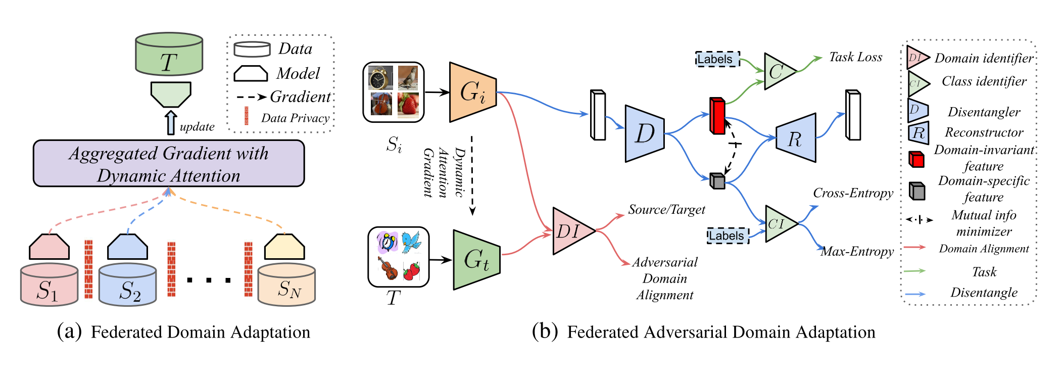
From the theory in the previous section, it is not difficult to see the importance of the weight and the distance. The method of this paper learns the weights by proposing a dynamic attention mechanism, and reduces the distance between the source domains and the target domain through a federated adversarial alignment mechanism. In addition, a feature disentanglement method is adopted to extract domain-invariant features to strengthen knowledge transfer.
Dynamic Attention Mechanism:
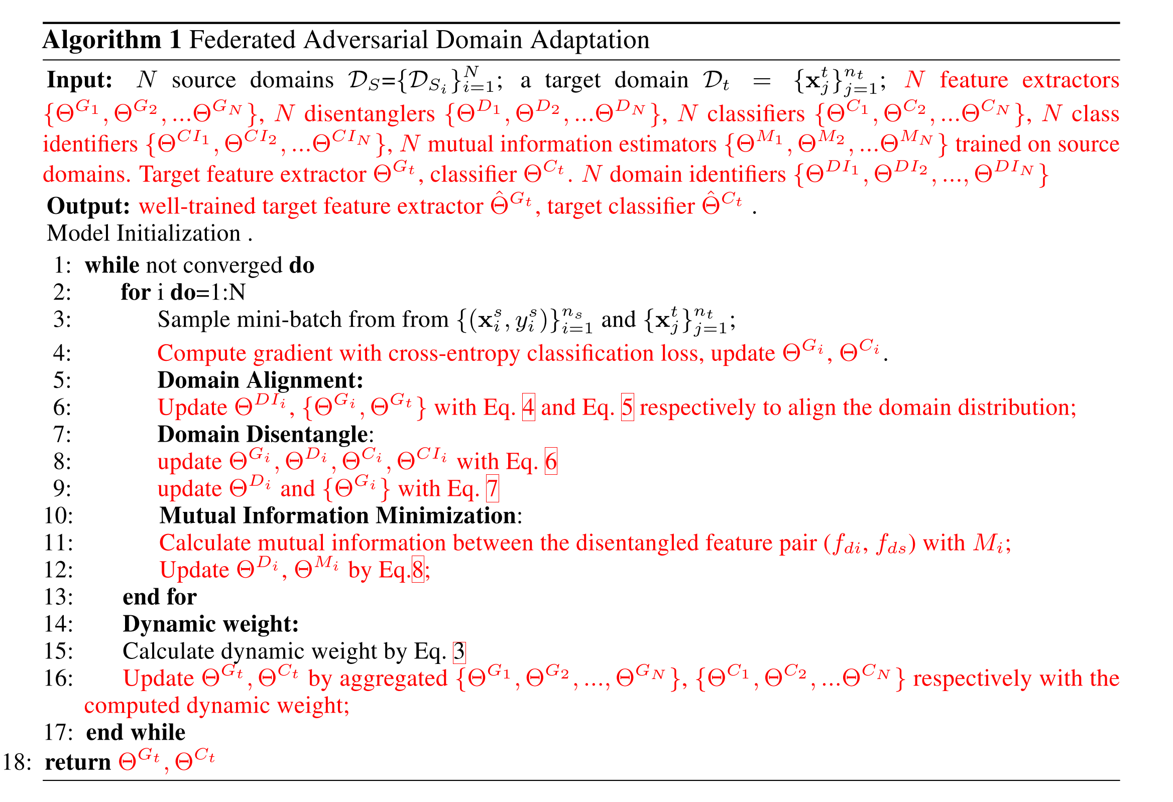
The principle of this mechanism is mainly to increase the weights of nodes with high contributions and decrease the weights of nodes with low contributions. So how do we judge the degree of a node’s contribution? This paper uses the gap statistics method to evaluate how well the target features can be clustered.
Assume there are clusters, where denotes the indices of the objects in the r-th cluster, and .
Intuitively, a smaller gap statistics value indicates that the feature distribution has smaller intra-class variance. The degree of contribution of each source node is measured by computing the difference between the gap statistics of two iterations.
It represents how much the clusters can be improved after the target domain is updated with a source domain’s gradient. For the gradient updates, the following is used to decide how much each gradient contributes:
Federated Adversarial Alignment:
Machine learning models can suffer greatly degraded performance due to domain distance. To solve this problem, this paper improves the traditional adversarial training method in the federated learning setting. In the federated learning context, this paper divides the adversarial alignment optimization process into two steps: 1. For each domain, train a local feature extractor, with and corresponding to and respectively. 2. For each () source-target domain pair, train an adversarial domain discriminator DI to align the two distributions in an adversarial learning way. First, train DI to recognize which feature domain a feature comes from; then train the generator, i.e., the feature extractors (), to fool DI. Note: D can only access the outputs of and .
Given the i-th source data domain and the target domain , the optimization objective of is:
Then, keeping D fixed, the objective function for updating G is:
Feature Disentanglement:
Under the adversarial learning framework, this paper also adopts adversarial disentanglement to extract domain-invariant features. The paper argues that the extracted features can be divided into domain-specific features and domain-invariant features. As shown in the first figure, the feature disentangler D divides the features into two categories. First, a K-class classifier and a K-class category recognizer are trained to predict labels from the features.
Then, with the category classifier fixed, only the feature disentangler is trained, producing domain-specific features to fool the category classifier.
The feature disentanglement method transfers knowledge by keeping the class-invariant features and removing the class-specific features. To enhance the disentanglement effect, this paper minimizes the mutual information between the two.
Mutual information is defined as , where is the joint probability distribution of the two kinds of features, and are the corresponding marginal probability distributions.
The Mutual Information Neural Estimator (MINE) is used to estimate the mutual information:
In practice, it can be computed by:
To avoid computing integrals, the Monte Carlo method is adopted:
where (p, q) are sampled from the joint distribution, is sampled from the marginal distribution, and is a neural network determined by that estimates the mutual information between the P and Q distributions.
The domain-invariant features and the domain-specific features are fed into a reconstructor to obtain recombined features; the loss function uses an L2 loss to reconstruct the original features, in order to preserve the composability of the representation. The L2 constraint and the mutual information loss constraint can be balanced by tuning the hyperparameters.
To be continued